H&M 데이터 분석(VS Code)

데이터에 대한 설명들

 

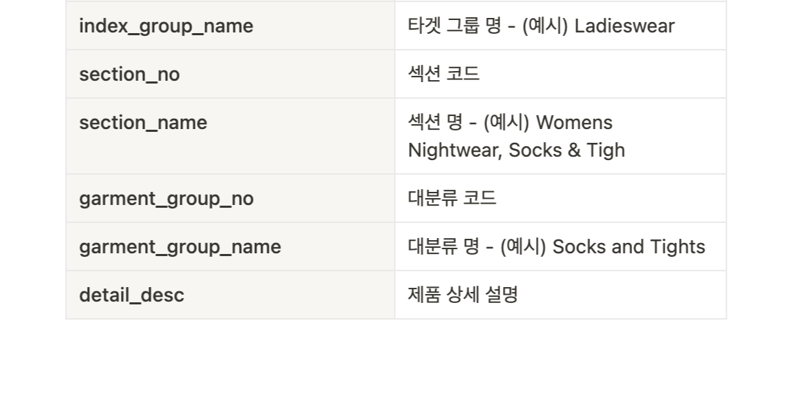
○컬럼들에 대한 설명

*article id: 특정 상품에 하나하나에 부여한 id

 

 

 

결측치 처리하는 것

 

https://velog.io/@cndbstlr7/%ED%8C%8C%EC%9D%B4%EC%8D%AC-%EA%B8%B0%EC%B4%88-4.-%EA%B2%B0%EC%B8%A1%EC%B9%98-%EC%B2%98%EB%A6%AC

파이썬 기초 4. 결측치 처리

https://rfriend.tistory.com/262

[Python pandas] 결측값 채우기, 결측값 대체하기, 결측값 처리 (filling missing value, imputation of missing valu

 

↑참고한 사이트들

 

***근데 결측치 처리할떄 원본을 복제해야함

안 그러면 이상한 컬럼들이 추가가 됨

 

#customer_df 결측치 0으로 채우기


clean_customer_df = customer_df.copy()  # 원본 유지
clean_customer_df['fashion_news_frequency'] = clean_customer_df['fashion_news_frequency'].fillna(0)

 

#Article_df 결측치 0으로 채우기: detail_desc

clean_article_df = article_df.copy()  # 원본 유지
clean_article_df['detail_desc'] = clean_article_df['detail_desc'].fillna(0)

 

↑이런식으로 하기

 

ARPU 구하기: Average Revenue Per User

총 매출 / 총 활성 사용자수

*활성 사용자는 구입 안 한 이들도 포함, 서비스나 어플을 사용한 이들

#Total users(그냥 가입한 사람들 다), 중복 없이 세기

customers = clean_customer_df['customer_id'].nunique()
customers



#total revenues(중복 있게 2번 이산 산것도 포함)

total_buy_rep = transaction_df['price'].sum()
total_buy_rep



#ARPU 구하기

arpu = total_buy_rep/customers_norep
arpu

 

ARPU: np.float64(0.027779152776233457)

 

돈 안 쓴 고객들도 포함해야 하니까 clean_customers_df(고객들에 대한 데이터를 갖고 있는 데이터)

 

 

ARPPU 구하기: Average Revenue Per Paying User

총 매출 / 총 유로 사용자

#결제를 한 user들만 보기


buy_customers_norep = transaction_df['customer_id'].nunique()
buy_customers_norep


#ARPPU 구하기

ARPPU = (total_buy_rep/buy_customers_norep)
ARPPU

 

ARPPU: np.float64(0.0635667836859668)

돈 쓴 고객들만 포함해야 하니까 transaction_df에 있는 customer_id 사용하기

 

https://kimsyoung.tistory.com/entry/ARPU%EC%99%80-ARPPU%EC%9D%98-%EC%B0%A8%EC%9D%B4

ARPU와 ARPPU의 차이?

ARPU, ARPPU구하는 것에 대하여 참고한 사이트

 

 

ARPU, ARPPU 값들 시각화하기

 

# 데이터
labels = ['ARPU', 'ARPPU']
values = [0.027779152776233457, 0.0635667836859668]


#색갈 설정
colors = ["green", "orange"]


# 그래프 그리기
bars = plt.bar(labels, values, color = colors)


# 제목과 레이블 추가
plt.title('ARPU, ARPPU Bar Graph')
plt.xlabel('Labels')
plt.ylabel('Values')


#막대에 숫자값 추가하기
plt.bar_label(bars, fmt="%.4f", label_type="edge", padding=-15, fontsize=12, fontweight='bold')


# 그래프 보이기
plt.show()

 

plt.bar_label(bars, fmt="%.4f", label_type="edge", padding=-15, fontsize=12, fontweight='bold')

 

fmt="%.4f": 소숫점 4번째 자리까지만 나오게 해줌

label_type="edge": 막대 꼭대기값에 표시

padding=-15: 막대 그래프 아래에 표시되게 해줌

fotsize=12, fontweight='bold': 글자 크기, 글자 모양

 

시각화한것↑

 

 

https://zephyrus1111.tistory.com/9

[바 차트(Bar chart)] 2. Matplotlib을 이용하여 바 차트 꾸미기

바 그래프  참고하기

 

 

구매 한 고객와, 구매 안 한 고객의 비율 구하기

 

○데이터부터 만들기

 

●구매한 고객만 나오게 데이터 만들기

#transaction, clean_customer_df join하기

tran_cus_df = pd.merge(clean_customer_df, transaction_df, on='customer_id', how='inner')

# customer_id 기준으로 중복 제거
tran_cus_df = tran_cus_df.drop_duplicates(subset='customer_id')

#구매한 고객만 나오는 데이터
tran_cus_df

 

●모든 고객이 다 나오게 데이터 구하기(중복 없에기)

#customer_id 중복 제거한 데이터: cus_dropdup_df
#모든 고객(구매를 한 고객과 안 한 고객)이 다 나옴

cus_dropdup_df = clean_customer_df.drop_duplicates(subset='customer_id')
cus_dropdup_df

 

○고객들에 대한 퍼센테이지 구하기

 

●구매 안 한 고객들에 대한 것

 

◎구매 안 한 고객수: 695015

#구매 안 한 고객 수

1048575-353560

 

전체 고객수의 데이터의 row수-구매한 고객수의 데이터의 row수

 

 

◎구매 안 한 고객의 비율: 66.28185871301528

# 구매 안 한 고객의 비율

(695015/1048575)*100

 

 

●구매 한 고객들에 대한 것

 

◎구매 한 고객의 수: 353560

# 구매 한 고객의 수

1048575-695015

 

 

◎구매 한 고객의 비율:33.71814128698472

# 구매 한 고객의 비율

(353560/1048575)*100

 

 

○구매한 고객들과 아닌 고객들에 대한 시각화 그래프

 

# 구매자들과, 구매 하지 않은 이들의 비율 시각화

people = ['buyers', 'non-buyers']
people_percentage = [33.7, 66.3]

plt.figure(figsize = (10, 5))
plt.pie(people_percentage, labels = people, autopct='%1.1f%%')  
plt.show()

 

autopct: 이 매개변수는 파이 차트의 각 조각에 표시할 값을 포맷하는 역할을 해

 

 

 

https://tnqkrdmssjan.tistory.com/58

[Python] Matplotlib 파이 차트 그리기

참고한 사이트

 

 

 

Box Plot 만들기(고객들의 주요 나이대를 알기 위해서 구하는것)

 

 

 

출처: https://bommbom.tistory.com/entry/%EB%B0%95%EC%8A%A4%ED%94%8C%EB%A1%AFBoxplox-%ED%95%B4%EC%84%9D%EA%B3%BC-%EC%82%AC%EC%9A%A9-%EB%B0%A9%EB%B2%95

박스플롯(Boxplox) 해석과 사용 방법

 

 

#고객들의 나이대 알기

plt.figure(figsize = (10, 5))
plt.boxplot([clean_customer_df['age']],\
            whis = 4, notch = True, vert = False)

plt.xticks(range(10, 101, 10)) 
plt.show()

 

plt.boxplot([clean_customer_df['age']],\whis = 4, notch = True, vert = False)

whis = 4: 수염 길이 조정

notch: 중앙값을 표시해줌

vert: 가로형으로 볼 수 있게 해줌

 

 

20대 초중반~40대 후반 사이의 고객들이 제일 많다

 

나이대별 고객들이 얼마나 있는지 시각화하기

# clean_customer_df데이터에서 'age'에서 그룹을 만들기(10대, 20대 이런식)

age_bins = list(range(10, 101, 10))  
age_labels = ['10s', '20s', '30s', '40s', '50s', '60s', '70s', '80s', '90s']

# 나이대를 범주형 변수로 변환

clean_customer_df['age_group'] = pd.cut(clean_customer_df['age'], bins=age_bins, labels=age_labels, right=True)

# 각 나이대별 개수 계산

age_counts = clean_customer_df['age_group'].value_counts().sort_index()

# 시각화하기
plt.figure(figsize=(10, 5))
plt.bar(age_counts.index, age_counts.values, color='skyblue', edgecolor='black')

# 그래프 제목, 축 라벨 설정
plt.title("Customer by age", fontsize=14)
plt.xlabel("Age", fontsize=12)
plt.ylabel("Customer", fontsize=12)
plt.xticks(rotation=45)
plt.grid(axis="y", alpha=0.7)

plt.show()

 

 

△clean_customer_df데이터에서 'age'에서 그룹을 만들기(10대, 20대 이런식)
▲age_bins = list(range(10, 101, 10))

10~100까지 10 단위로(10,20,30 이런식) 숫자들 생성

▲age_labels = ['10s', '20s', '30s', '40s', '50s', '60s', '70s', '80s', '90s']

 

△clean_customer_df['age_group'] = pd.cut(clean_customer_df['age'], bins=age_bins, labels=age_labels, right=False)

▲pd.cut: 연속적인 숫자들은 구간에 맞게 나누기

ex: 10, 15, 16, 29, 27, 30,34

10대: 10,15,16

20대: 29,27

30대: 30,34

▲clean_customer_df['age']: clean_customer_df데이터에서 age컬럼을 기준으로 나눈다

▲right-True

10~19까지 다 포함되게 설정

 

△age_counts = clean_customer_df['age_group'].value_counts().sort_index()

▲sort_index(): 오름차순으로 해줌

 

△plt.grid(axis="y", alpha=0.7)

▲axis="y": y축에 그리도 표시, alpha=0.7:투명도 설정

 

 

 

Club Member Status(회원 상태), Age별  Price(가격-매출) 보기

 

○데이터 만들기

# customer_id를 기준으로 transaction_df, clean_customer_df merge

merged_df = clean_customer_df.merge(transaction_df, on='customer_id', how='inner')

price만 transactions_df에 있어서 merge 씀

transactions_df, clean_customer_df 공통적으로 customer_id 컬럼은 있음

 

△Merge 형태

merged_df = 첫 번째 데이터.merge(두 번째 데이터, on='공통 컬럼', how='병합 방식')

 

▲첫 번째 데이터

 

▲두 번째 데이터: 추가 정보

 

 

○ 나이대별 status에 따른 매출 구해보기-시각화

 

●Age에 따른 그룹 만들기

# clean_customer_df데이터에서 'age'에서 그룹을 만들기(10대, 20대 이런식)
# 위와 똑같은데 에러가 생길수 있어서 이름만 변경

age_bins_2 = list(range(10, 101, 10))  
age_labels_2 = ['10s', '20s', '30s', '40s', '50s', '60s', '70s', '80s', '90s']

# 나이대를 범주형 변수로 변환

clean_customer_df['age_group'] = pd.cut(clean_customer_df['age'], bins=age_bins_2, labels=age_labels_2, right=True)

 

위와 똑같은것

이름이 같을시 에러가 날 수 있으니까 데이터들의 이름만 바꿈

 

 

●나이대별, status별 매출 합계 구하기

# 나이대별, status별 매출 합계 구하기

sales_by_age_status = merged_df.groupby(['age_group', 'club_member_status'])['price'].sum().unstack()

 

merged_df데이터를 기준(다음에 나올 컬럼들이 속한 데이터를 쓰는 자리)으로 age_group, club_member_status컬럼을 그룹화한뒤 price의 sum을 구함

 

unstack을 써야 status의 종류별로 볼 수 있음

 

●최종적으로 시각화

#시각화하기

# 그래프 크기 설정
plt.figure(figsize=(10, 6))

# 나이대와 상태별 매출 시각화
sales_by_age_status.plot(kind='bar', stacked=False, colormap='viridis', edgecolor='black', figsize=(10, 6))

# 그래프 제목들과 label들 설정
plt.title("Sales by Age Group and Club Member Status", fontsize=14)
plt.xlabel("Age Group", fontsize=12)
plt.ylabel("Total Sales", fontsize=12)
plt.xticks(rotation=45)  
plt.legend(title="Status") 
plt.grid(axis="y", alpha=0.7)

# 그래프 나오게 하기
plt.show()

 

▲나이대와 상태별 매출 시각화

△Stacked=False: 그룹형 막대 그래프

 

▲그래프 제목들과 label들 설정

△plt.grid(axis="y", alpha=0.7): y축 방향으로 선 추가

 

 

모든 나이대별 모든 유저들의 status는 Active하다, 매우 소수만 pre-create

 

 

오프라인/온라인 구매 빈도수와 총합

 

○대이터 만들기

 

# customer_id를 기준으로 transaction_df, clean_customer_df merge

article_tran_merged_df = clean_article_df.merge(transaction_df, on="article_id", how="inner")

 

 

 

○오프라인 구매 빈도수, 총합

 

#오프라인 판매에 대해
#1=오프라인

#얼마나 많이 나타나는지
count_off = (article_tran_merged_df["sales_channel_id"] == 1).sum()
print(count_off)

#오프라인 판매의 총합
off_total_price = article_tran_merged_df[article_tran_merged_df["sales_channel_id"] == 1]["price"].sum()
print(off_total_price)

 

# 오프라인 데이터
labels = ['Offline Frequency', 'Offline Total Price']
values = [319383, 7284.189344698002]

#색갈 설정
colors = ["green", "orange"]

# 그래프 그리기
bars = plt.bar(labels, values, color = colors)

# 제목과 레이블 추가
plt.title('Offline Bar Graph')
plt.xlabel('Offline')
plt.ylabel('Amount')

#막대에 숫자값 추가하기
plt.bar_label(bars, fmt="%.4f", label_type="edge", padding=-1, fontsize=12, fontweight='bold')

# 그래프 보이기
plt.show()

 

 

○온라인 구매 빈도수, 총합

 

#온라인 판매에 대해
#2=온라인

#얼마나 많이 나타나는지
count_on = (article_tran_merged_df["sales_channel_id"] == 2).sum()
print(count_on)

#오프라인 판매의 총합
on_total_price = article_tran_merged_df[article_tran_merged_df["sales_channel_id"] == 2]["price"].sum()
print(on_total_price)

 

# 온라인 데이터
labels = ['Online Frequency', 'Online Total Price']
values = [729192, 21844.335777640998]

#색갈 설정
colors = ["green", "orange"]

# 그래프 그리기
bars = plt.bar(labels, values, color = colors)

# 제목과 레이블 추가
plt.title('Online Bar Graph')
plt.xlabel('Online')
plt.ylabel('Amount')

#막대에 숫자값 추가하기
plt.bar_label(bars, fmt="%.4f", label_type="edge", padding=-1, fontsize=12, fontweight='bold')

# 그래프 보이기
plt.show()

 

 

고객들이 많이/적게 한 연도/달

 

# article_tran_merged_df 데이터에서 t_dat컬럼 월, 달 따로 빼서 새로운 컬럼 만들기

article_tran_merged_df['year'] = pd.to_datetime(article_tran_merged_df['t_dat']).dt.year  
article_tran_merged_df['month'] = pd.to_datetime(article_tran_merged_df['t_dat']).dt.month

연도, 달별 보기 위해서 따로 달과 연도만 뺀 컬럼 만듬

 

#year에서는 총 몇가지의 value들이 있는지 보기

article_tran_merged_df['year'].value_counts()

2019년만 나와서 연도는 따로 안 볼 예정

 

 

오프라인, 온라인으로 산거 다 합쳐진 각 달별 매출 총합 시각화

 

#모든 방법(offline, online) 달별 총매출

all_month_sales_sum = article_tran_merged_df.groupby('month')['price'].sum()
all_month_sales_sum

# 월별 매출 합계 구하기: 전체 데이터
month_sum_price = article_tran_merged_df.groupby('month')['price'].sum()

# 매출 합계를 기준으로 내림차순 정렬: 매출이 큰 달부터 나오게 하기
month_sum_price_sorted = month_sum_price.sort_values(ascending=False)

# 그래프 크기 설정
plt.figure(figsize=(8, 5))

# 시각화하기
sns.barplot(x=month_sum_price_sorted.index, y=month_sum_price_sorted.values, order=month_sum_price_sorted.index)

# 제목, 라벨 설정
plt.title("Total Sales by Month (all)")
plt.xlabel("Month")
plt.ylabel("Total Sales")

# 그래프 출력
plt.show()

 

 

 

달별 오프라인 매출: 오프라인

 

# 오프라인 데이터만 보기
off_filtered_data = article_tran_merged_df[article_tran_merged_df['sales_channel_id'] == 1]

# 오프라인 월별 매출
offline_month_sales = off_filtered_data.groupby('month')['price'].sum()
offline_month_sales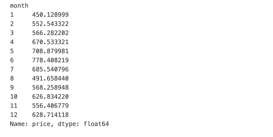

#1=오프라인
#달별 오프라인 매출보기

# id가 1인 데이터만 필터링
filtered_1_data = article_tran_merged_df[article_tran_merged_df['sales_channel_id'] == 1]

# 월별 매출 합계 구하기
month_sum_price = filtered_1_data.groupby('month')['price'].sum()

# 매출 합계를 기준으로 내림차순 정렬
month_sum_price_sorted = month_sum_price.sort_values(ascending=False)

# 그래프 크기 설정
plt.figure(figsize=(8, 5))

# 막대그래프 그리기
sns.barplot(x=month_sum_price_sorted.index, y=month_sum_price_sorted.values, order=month_sum_price_sorted.index)

# 그래프 제목 및 라벨 설정
plt.title("Total Offline Sales by Month")
plt.xlabel("Month")
plt.ylabel("Total Sales")

# 그래프 출력
plt.show()

 

 

 

 

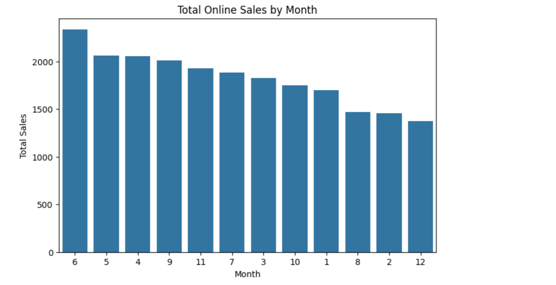
달별 온라인 매출

# 온라인 데이터만 보기
on_filtered_data = article_tran_merged_df[article_tran_merged_df['sales_channel_id'] == 2]

# 온라인 월별 매출
on_month_sales = on_filtered_data.groupby('month')['price'].sum()
on_month_sales

#2=online
#달별 온라인 매출의 총액

# id가 2인 데이터만 필터링
filtered_2_data = article_tran_merged_df[article_tran_merged_df['sales_channel_id'] == 2]

#달별 총매출 
month_sum_price = filtered_2_data.groupby('month')['price'].sum()

# 매출 합계를 기준으로 내림차순 정렬
month_sum_price_sorted = month_sum_price.sort_values(ascending=False)

# 그래프 크기 설정
plt.figure(figsize=(8, 5))

# 막대그래프 그리기
sns.barplot(x=month_sum_price_sorted.index, y=month_sum_price_sorted.values, order=month_sum_price_sorted.index)

# 그래프 제목 및 라벨 설정
plt.title("Total Online Sales by Month")
plt.xlabel("Month")
plt.ylabel("Total Sales")

# 그래프 출력
plt.show()

 

 

 

어떤 물건+색의 조합이 가장 많이 팔렸는지(온/오프라인 다 합쳐서)

# 매출 합계로 그룹화하고 상위 15개만 추출(다 있는거)

top5 = article_tran_merged_df.groupby(['product_type_name', 'perceived_colour_master_name'])['price'].sum().nlargest(15)

# 바 차트로 시각화

top5.plot(kind='barh', color='skyblue', figsize=(10, 6))
plt.xlabel('Total Sales Made')
plt.title('Top 15 Sales of Products & Color')
plt.show()

 

어떤 물건+색의 조합이 가장 많이 팔렸는지(오프라인만)

 

# 오프라인 데이터 필터링

df_filtered_offline = article_tran_merged_df[(article_tran_merged_df['sales_channel_id'] == 1)]

# 상위 15개의 옷 종류+색만 추출

top5 = df_filtered_offline.groupby(['product_type_name', 'perceived_colour_master_name'])['price'].sum().nlargest(15)

# 바 차트로 시각화

top5.plot(kind='barh', color='skyblue', figsize=(10, 6))
plt.xlabel('Total Sales Made')
plt.title('Top 15 Offline Sales of Products & Color')
plt.show()

 

어떤 물건+색의 조합이 가장 많이 팔렸는지(온라인만)

# 온라인 데이터 필터링

df_filtered = article_tran_merged_df[(article_tran_merged_df['sales_channel_id'] == 2)]

# 상위 15개의 옷 종류+색만 추출

top5 = df_filtered.groupby(['product_type_name', 'perceived_colour_master_name'])['price'].sum().nlargest(15)

# 바 차트로 시각화

top5.plot(kind='barh', color='skyblue', figsize=(10, 6))
plt.xlabel('Total Sales Made')
plt.title('Top 15 Online Sales of Products & Color')
plt.show()